One landmark theorem in Financial Economics is the Efficient Market Hypothesis (EMH). This theorem posits that in an arbitrage-free market, we can model an asset’s present price as the discounted expected future price:
![{\displaystyle P_{t}=ME_{t}[P_{t+1}]}](https://wikimedia.org/api/rest_v1/media/math/render/svg/61acd66b4700ffc07c80c08754b32c27a5442faf)
We can take the natural logarithm
![{\displaystyle \log P_{t}=\log M+E_{t}[\log P_{t+1}]}](https://wikimedia.org/api/rest_v1/media/math/render/svg/2d429b682b19a6680a1b66fb544382af47a78d2e)
to show that the natural logarithm of asset prices follows a random walk – the best forecast for prices is simply the current price. As such, applying regression methods from basic ARIMA models to advanced neural networks will fail – the models will simply repeat the last observation in the training data.
Instead, we can successfully predict asset prices by assuming their returns follow Geometric Brownian Motion (GBM):

Here, the change in returns is given by the expected value plus volatility, both multiplied by the last observed price. For the log of returns, and using Ito’s Lemma, one can write the solution to this differential equation as

where B_t represents a Brownian motion process. The above formula is how we will forecast liquid asset prices in this article. For models in other asset types (ie illiquid assets), one may simply substitute the GBM equation in Ito’s Lemma and derive a new formula for forecasting.
We first import our packages:
import pandas as pd
import matplotlib.pyplot as plt
import numpy as np
import scipy
from fitter import Fitter
For today, we forecast Bitcoin using data from August 01, 2020 to November 15, 2021. Our data comes from Yahoo Finance.
liquid = pd.read_csv("/path/to/BTC-USD.csv")
liquid_returns = np.log(liquid.Close) - np.log(liquid.Close.shift(1))
We split both our returns and prices data into training and testing sets:
train, test = pmdarima.model_selection.train_test_split(liquid.Close.dropna(), train_size = 0.8)
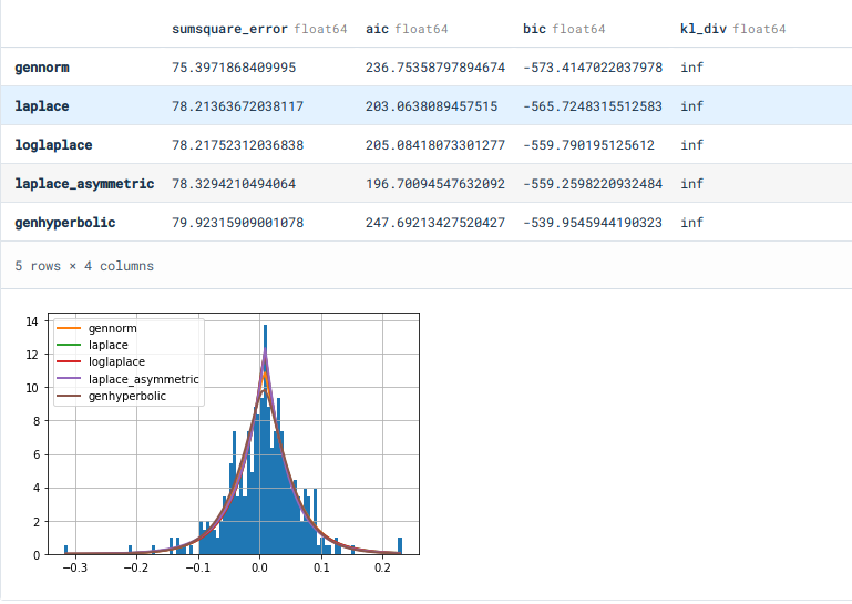
training, testing = pmdarima.model_selection.train_test_split(liquid_returns.dropna(), train_size = 0.8)Now, we obtain the distribution of our returns. Note that it is a common and erroneous practice to assume that returns follow a normal distribution in forecasting. This practice yields disastrous results – one needs proper knowledge of the distribution to forecast properly.
f = Fitter(training, timeout = 120)
f.fit()
f.summary()
Using BIC as our criterion, we get the Laplace distribution as our best distribution.
f.get_best(method = "bic")We now write our main function for performing Monte Carlo Integration. This methods uses random numbers to repeatedly sample future results – in our case, we sample random numbers from a Laplace Distribution, then multiply them to our volatility to obtain our diffusion term.
def GBMsimulatorUniVar(So, mu, sigma, T, N):
    dim = np.size(So)
    S = np.zeros([T + 1, int(N)])
    S[0, :] = So
    for t in range(1, int(T) + 1):
        for i in range(0, int(N)):
            drift = (mu - 0.5 * sigma**2)
            Z = scipy.stats.laplace.rvs()
            diffusion = sigma*Z
            S[t][i] = S[t - 1][i]*np.exp(drift + diffusion)
    return S[1:]
Here, we forecast our prices with 1000 simulations for the length of our testing data. We use the average of simulations as our optimal forecast.
prices = GBMsimulatorUniVar(So = liquid.Close.iloc[len(training)], mu = training.mean(), sigma = training.std(), T = len(test), N = 1000)
newpreds = pd.DataFrame(prices).mean(axis = 1)
Taking the mean average prediction error (MAPE), we find around 6.8% forecasting error.
from sklearn.metrics import mean_absolute_percentage_error as mape
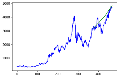
mape(newpreds, test.dropna())We now plot our forecast against the real test values.
axis = np.arange(len(train) + len(test))
plt.plot(axis[:len(train)], train, c = "blue")
plt.plot(axis[len(train):], test, c = "blue")
plt.plot(axis[len(train):], np.array(newpreds), c = "green")
As one can see, we have relatively good results.
One should note that other assets may have different distributions. For instance, here are distribution fit results for Ethereum:
> f.get_best(method = "bic")
{'gennorm': {'beta': 1.126689300086524,
  'loc': 0.007308884923027554,
  'scale': 0.047110827282059724}}
As a rule of thumb, the distribution parameters in the fit function need to be multiplied by 2.5 when sampling random numbers to obtain good forecast results. One must also use common sense in determining which proposed distribution to use – those such as the Gumbel, Logistic, or similar ones (used to model categorical data) are wholly unsuitable for stock price data.
def GBMsimulatorUniVar(So, mu, sigma, T, N):
    dim = np.size(So)
    #t = np.linspace(0., T, int(N))
    S = np.zeros([T + 1, int(N)])
    S[0, :] = So
    for t in range(1, int(T) + 1):
        for i in range(0, int(N)):
            drift = (mu - 0.5 * sigma**2)
            Z = scipy.stats.gennorm.rvs(beta = 1.126689300086524*2.5)
            diffusion = sigma*Z
            S[t][i] = S[t - 1][i]*np.exp(drift + diffusion)
    return S[1:]#, t
This forecast obtains around 8.6% forecasting error with Ethereum.
While some asset prices may follow random walks, using the proper tools to model them gives great forecasting results and accuracy. However, even with the best tools and distributions, no forecast will ever be great if a structural break exists in the data. Both our Ethereum and Bitcoin data started and ended during the COVID-19 Pandemic – mixing pre and post pandemic data is always an ill-advised move.
Super helpful – thank you!
Brownian motion is SUPER tractable analytically, why would I be interested in a computational treatment with its inherent lack of generality when there’s likely an analytical paper with more robust insights?
If you’re not interested why are you on this page? You’re not the audience for this article.