As we saw in other econometric blogs of M&S Research Hub, the use of logarithms constitutes a usual practice in econometrics, not only for the problems that can be derived from overusing them, but also it was mentioned the advantage to reduce the Heteroscedasticity -HT- (Nau, 2019) present in the series of a dataset, and some improvements that the monotonic transformation performs on the data as well.
In this article, we’re going to explore the utility of the logarithm transformation to reduce the presence of structural breaks in the time series context. First, we’ll review what’s a structural break, what are the implications of regressing data with structural breaks and finally, we’re going to perform a short empirical analysis with the Gross Domestic Product -GDP- of Colombia in Stata.
The structural break
We can define a structural break as a situation where a sudden, unexpected change occurs in a time series variable, or a sudden change in the relationship between two-time series (Casini & Perron, 2018). In this order of ideas, a structural change might look like this:

The basic idea is to identify abrupt changes in time series variables but we’re not restricting such identification to the domain of time, it can be detected also when we scatter X and Y variables that not necessarily consider the dependent variable as the time. We can distinguish different types of breaks in this context, according to Hansen (2012) we can encounter breaks in 1) Mean, 2) Variance, 3) Relationships, and also we can face single breaks, multiple breaks, and continuous breaks.
Basic problems of the structural breaks
Without going into complex mathematical definitions of the structural breaks, we can establish some of the problems when our data has this situation. The first problem was identified by Andrews (1993) regarding to the parameter’s stability related to structural changes, in simple terms, in the presence of a break, the estimators of the least square regression tend to vary over time, which is of course something not desirable, the ideal situation is that the estimators would be time invariant to consolidate the Best Linear Unbiased Estimator -BLUE-.
The second problem of structural breaks (or changes) not taken in account during the regression analysis is the fact that the estimator turns to be inefficient since the estimated parameters are going to have a significant increase in the variance, so we’re not getting a statistical unbiased estimator and our exact inferences or forecasting analysis wouldn’t be according to reality.
A third problem might appear if the structural break influences the unit root identification process, this is not a wide explored topic but Tai-Leung Chong (2001) makes excellent appoints related to this. Any time series analysis should always consider the existence of unit roots in the variables, in order to provide further tools to handle a phenomenon, that includes the cointegration field and the forecasting techniques.
An empirical approximation
Suppose we want to model the tendency of the GDP of the Colombian economy, naturally this kind of analysis explicitly takes the GDP as the dependent variable, and the time as the independent variable, following the next form:

In this case, we know that the GDP expressed in Y is going to be a function of the time t. We can assume for a start that the function f(t) follows a linear approximation.

With this expression in (1), the gross domestic production would have an independent autonomous value independent of time defined in a, and we’ll get the slope coefficient in α which has the usual interpretation that by an increase of one-time unit, the GDP will have an increase of α.
The linear approximation sounds ideal to model the GDP against the changes over time, assuming that t has a periodicity of years, meaning that we have annual data (so we’re excluding stational phenomena); however, we shall always inspect the data with some graphics.
With Stata once we already tsset the database, we can watch the graphical behavior with the command “scatter y t”.


In sum, the linear approximation might not be a good idea with this behavior of the real GDP of the Colombian economy for the period of analysis (1950-2014). And it appears to be some structural changes judging by the tendency which changes the slope of the curve drastically around the year 2000.
If we regress the expression in (1), we’ll get the next results.

The linear explanation of the time (in years) related to the GDP is pretty good, around 93% of the independent variable given by the time, explains the GDP of the Colombian economy, and the parameter is significant with a level of 5%.
Now I want you to focus in two basic things, the variance of the model which is 1.7446e+09 and the confidence intervals, which positions the estimator between 7613.081 and 8743.697. Without having other values to compare these two things, we should just keep them in mind.
Now, we can proceed with a test to identify structural breaks in the regression we have just performed. So, we just type “estat sbsingle” in order to test for a structural break with an unknown date.

The interesting thing here is that the structural break test identifies one important change over the full sample period of 1950 to 2014, the whole sample test is called “supremum Wald test” and it is said to have less power than average or exponential tests. However, the test is useful in terms of simply identify structural terms which also tend to match with the graphical analysis. According to the test, we have a structural break in the year 2002, so it would be useful to graph the behavior before and after this year in order to conclude the possible changes. We can do this with the command “scatter y t” and include some if conditions like it follows ahead.
twoway (scatter Y t if t<=2002)(lfit Y t if t<=2002)(scatter Y t if t>=2002)(lfit Y t if t>=2002)
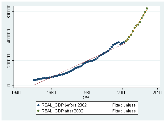
We can observe that tendency is actually changing if we adjust the line for partial periods of time, given by t<2002 and t>2002, meaning that the slope change is a sign of structural break detected by the program. You can attend this issue including a dummy variable that would equal 0 in the time before 2002 and equal 1 after 2002. However, let’s graph now the logarithm transformation of GDP. The mathematical model would be:

Applying natural logarithms, we got:

α now becomes the average growth rate per year of the GDP of the Colombian economy, to implement this transformation use the command “gen ln_y=ln(Y)” and the graphical behavior would look like this:
 gen ln_Y=ln(Y)
 scatter ln_Y t

The power of the monotonic transformation is now visible, there’s a straight line among the variable which can be fitted using a linear regression, in fact, let’s regress the expression in Stata.
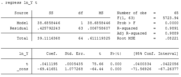
Remember that I told you to keep in mind the variance and the confidence intervals of the first regression? well now we can compare it since we got two models, the variance of the last regression is 0.0067 and the intervals are indeed close to the coefficient (around 0.002 of difference between the upper and lower interval for the parameter). So, this model fits even greatly than the first.
If we perform again the “estat sbsingle” test again, it’s highly likely that another structural break might appear. But we should not worry a lot if this happens, because we rely on the graphical analysis to proceed with the inferences, in other words, we shall be parsimonious with our models, with little, explain the most.
The main conclusion of this article is that the logarithms used with its property of monotonic transformation constitutes a quick, powerful tool that can help us to reduce (or even delete) the influences of structural breaks in our regression analysis. Structural changes are also, for example, signs of exogenous transformation of the economy, as a mention to apply this idea for the Colombian economy, we see it’s growing speed changing from 2002 until the recent years, but we need to consider that in 2002, Colombia faced a government change which was focused on the implementation of public policies related to eliminating terrorist groups, which probably had an impact related to the investment process in the economy and might explain the growth since then.
Bibliography
Andrews, D. W. (1993). Tests for Parameter Instability and Structural Change With Unknown Change Point. Journal of the Econometric Society Vol. 61, No. 4 (Jul., 1993), 821-856.
Casini, A., & Perron, P. (2018). Structural Breaks in Time Series. Retrieved from Economics Department, Boston University: https://arxiv.org/pdf/1805.03807.pdf
Hansen, B. E. (2012). Advanced Time Series and Forecasting. Retrieved from Lecture 5 tructural Breaks. University of Wisconsin Madison: https://www.ssc.wisc.edu/~bhansen/crete/crete5.pdf
Nau, R. (2019). The logarithm transformation. Retrieved from Data concepts The logarithm transformation: https://people.duke.edu/~rnau/411log.htm
Shresta, M., & Bhatta, G. (2018). Selecting appropriate methodological framework for time series data analysis. Retrieved from The Journal of Finance and Data Science: https://www.sciencedirect.com/science/article/pii/S2405918817300405
Tai-Leung Chong, T. (2001). Structural Change In Ar(1) Models. Retrieved from Econometric Theory,17. Printed in the United States of America: 87–155
Hi there! I simply would like to offer you a huge thumbs up for your great information you’ve got right here on this post. I’ll be returning to your website for more soon.
It’s hard to come by experienced people about this subject, however, you sound like you know what you’re talking about! Thanks
Hmm is anyone else experiencing problems with the pictures on this blog loading? I’m trying to determine if its a problem on my end or if it’s the blog. Any suggestions would be greatly appreciated.