Regarding microeconometrics, we can find applications that go from latent variables to model market decisions (like logit and probit models) and techniques to estimate the basic approaches for consumers and producers.
In this article, I want to start with an introduction of a basic concept in microeconomics, which is the Cobb-Douglas utility function and its estimation with Stata. So we’re reviewing the basic utility function, some mathematical forms to estimate it and finally, we’ll see an application using Stata.
Let’s start with the traditional Cobb-Douglas function:

Depending on the elasticity α and β for goods X and Y, we’ll have a respective preference of the consumer given by the utility function just above. In basic terms, we restrict α + β =1 in order to have an appropriate utility function which reflects a rate of substitution between the two goods X and Y. If we assume a constant value of the utility given by U* for the consumer, we could graph the curve by solving the equation for Y, in this order of ideas.

And the behavior of the utility function will be given by the number of quantities of the good Y explained by X and the respective elasticities α and β. We can graph the behavior of the indifference curve given a constant utility level according to the quantities of X and Y, also for a start, we will assume that α =0.5 and β=0.5 where the function has the following pattern for the same U* level of utility (example U=10), this reflects the substitution between the goods.
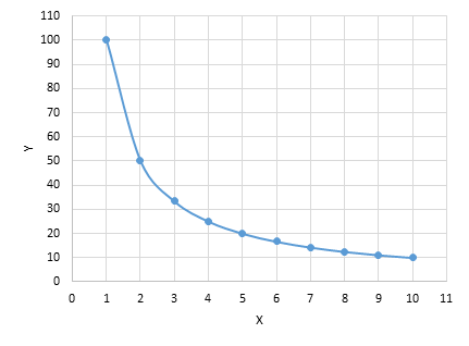
If you might wonder what happens when we alter the elasticity of each good, like for example, α =0.7 and β=0.3 the result would be a fast decaying curve instead of the pattern of the utility before.

Estimating the utility function of the Cobb-Douglas type will require data of a set of goods (X and Y in this case) and the utility.
Also, it would imply that you somehow measured the utility (that is, selecting a unit or a measure for the utility), sometimes this can be in monetary units or more complex ideas deriving from subjective utility measures.
Applying logarithms to the equation of the Cobb-Douglas function would result in:

Which with properties of logarithms can be expressed as:

This allows a linearization of the function as well, and we can see that the only thing we don’t know regarding the original function is the elasticities of α and β. The above equation fits perfectly in terms of a bivariate regression model. But remember to add the stochastic part when you’re modeling the function (that is, including the residual in the expression). With this, we can start to do a regressing exercise of the logarithm of the utility for the consumers taking into account the amount of the demanded goods X and Y. The result would allow us to estimate the behavior of the curve.

However, some assumptions must be noted: 1) We’re assuming that our sample (or subsample) containing the set of individuals i tend to have a similar utility function, 2) the estimation of the elasticity for each good, would also be a generalization of the individual behavior as an aggregate. One could argue that each individual i has a different utility function to maximize, and also that the elasticities for each good are different across individuals. But we can argue also that if the individuals i are somewhat homogenous (regarding income, tastes, and priorities, for example, the people of the same socioeconomic stratum) we might be able to proceed with the estimation of the function to model the consumer behavior toward the goods.
The Stata application
As a first step would be to inspect the data in graphical terms, scatter command, in this case, would be useful since it displays the behavior and correlation of the utility (U) and the goods (X and Y), adding some simple fitting lines the result would be displayed like this:
twoway scatter U x || lfit U x
twoway scatter U y || lfit U y
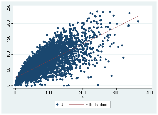
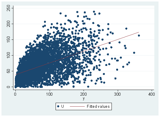
Up to this point, we can detect a higher dispersion regarding good Y. Also, the fitted line pattern relative to the slope is different for each good. This might lead to assume for now that the overall preference of the consumer for the n individuals is higher on average for the X good than it is for the Y good. The slope, in fact, is telling us that by an increase of one unit in the X good, there’s a serious increase in the utility (U) meanwhile, the fitted line on the good Y regarding to its slope is telling us comparatively speaking, that it doesn’t increase the utility as much as the X good. For this cross-sectional study, it also would become more useful to calculate Pearson’s correlation coefficient. This can be done with:
correlate U y x
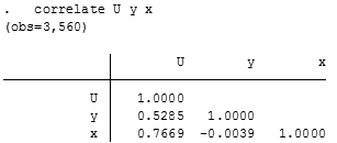
The coefficient is indicating us that exists somewhat of a linear association between the utility (U) and the good Y, meanwhile, it exists a stronger linear relationship relative to the X good and the utility. As a final point, there’s an inverse, but not significant or important linear relationship between goods X and Y. So the sign is indicating us that they’re substitutes of each other.
Now instead of regressing U with X and Y, we need to convert it into logarithms, because we want to do a linearization of the Cobb-Douglas utility function.
gen ln_U=ln(U)
gen ln_X=ln(x)
gen ln_Y=ln(y)
reg ln_U ln_X ln_Y
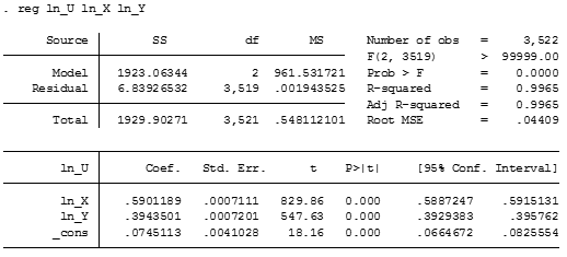
And now performing the regression without the constant.

Both regressions (with and without the constant) tends to establish the parameters in α =0.6 and β=0.4 which matches the Data Generating Process of the Montecarlo simulation. It appears that the model with the constant term has a lesser variance, so we shall select these parameters for further analysis.
How would it look then our estimation of this utility function for our sample? well, we can start using the mean value of the utility using descriptive statistics and then use a graphical function with the parameters associate. Remember that we got:

And we know already the parameters and also we can assume that the expected utility would be the mean utility in our sample. From this, we can use the command:
sum U y x

And with this, the estimated function for the utility level U=67.89 with approximated elasticities of 0.6 and 0.4 would look like this:

In this order of ideas, we just estimated the indifference curve for a certain population which consists of a set of i individuals. The expected utility from both goods was assumed as the mean value of the utility for the sample and with this, we can identify the different sets of points related to the goods X and Y which represents the expected utility. This is where it ends our brief example of the modeling related to the Cobb-Douglas utility function within a sample with two goods and defined utilities.
Interesting, keep it up.
hello 🙂 I am fond of the internet economy!
It’s very easy to find out any matter on net as
compared to textbooks, as I found this paragraph
at this web site.
Great article. When you launch into the Stata bit, I think you forgot to mention what you use as a data source. Without that, it’s hard to “follow along” and get the intuition of it all. Thanks!
Greetings, Thank you for your comment. Yes, I’ve forgotten to include the source of the data. For this post, it was a simulation. Although it will not be the same (I forgot which was the seed generated by that exercise) the code to generate the dataset is giving by:
set seed 1234
set obs 3560
gen y=abs(rnormal())
gen x=abs(rnormal())
gen U=(y^0.6)*(x^0.4)+rnormal()
With this you’ll have sort of the same exercise !
Thank you for this very good posts. I was wanting to know whether
you were planning of publishing similar posts
to this. Keep up writing superb content articles!
It is not my first time to pay a visit this web site,
i am visiting this website dailly and take pleasant data from here everyday.
With thanks for sharing your supertb website!
I join. I agree with all of the above. Let’s discuss this issue.
After study just a few of the blog posts in your website now, and I truly like your method of blogging. I bookmarked it to my bookmark website record and will likely be checking back soon. Pls try my web site as properly and let me know what you think.
you could have a fantastic weblog here! would you wish to make some invite posts on my weblog?
Hi
Thank you for this research .
My comment ..
Can You estimated Potential GDP by cobb doclas function..if you can ,what’s the deferential between tha suggest above, and others method, for example;by filtering HP the real GDP..
Thanks.
The Cobb-Douglas utility function that it’s exposed here has a more microeconomic approach. The one you’re mentioning is the aggregate production function of the form Y=K^(α) B^(1-α). It is widely use to model the importance of the elasticity regarding the factors of Capital K and Labor L.
However potential GDP is normally estimated with filters as you mention (Kalman filter might be able to help you to model with the Cobb-Douglas). Actually real applications for the TFP (Total Factor Productivity) are used with a smooth path of the filter for the Solow’s residual.
I suggest you stick parsimonious when you’re estimating anything econometrically. So if you take the Hodrick-Prescott filter to the real GDP (and adjusting the parameter lambda to your periodicity) you’ll have an approximation of the potential GDP in the long-run.