We mentioned in the last post the Solow-Swan model in order to explain the importance of the specification related to theories and the regression analysis. In this post, I’m going to explain a little bit more the neoclassical optimization related to consumption, in this case, it’s going to be fundamental to the theory of Ramsey (1928) related to the behavior of savings & consumption.
We declare first some usual assumptions, like closed economy XN=0, net investment equals I=K-δK where δ is a common depreciation rate of the economy for all kinds of capital. There’s no government spending in the model so G=0. And finally, we’re setting a function which is going to capture the individual utility u(c) given by:

This one is referred to as the constant intertemporal elasticity function of the consumption c over time t. The behavior of this function can be established as:
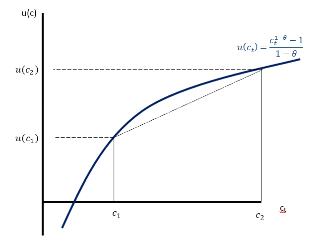
This is a utility function with a concave behavior, basically, as consumption in per capita terms is increasing, the utility also is increasing, however, the variation relative to the utility and the consumption is decreasing until it gets to a semi-constant state, where the slope of the points c1 and c2 is going to be decreasing.
We can establish some results of the function here, like

And that
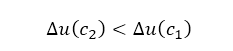
That implies that the utility at a higher consumption point is bigger than on a low consumption point, but the variation of the points is decreasing every time.
The overall utility function for the whole economy evaluated at a certain time can be written as:
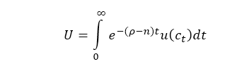
Where U is the aggregated utility of the economy at a certain time (t=0), e is the exponential function, ρ is the intergenerational discount rate of the consumption (this one refers to how much the individuals discount their present consumption related to the next generations) n is the growth rate of the population, t is the time, and u(c) is our individual utility function, dt is just the differential which indicates what are we integrating.
Think of this integral as a sum. You can aggregate the proportion of individual utilities at a respective time considering the population size, but also you need to bring back to the present the utility of other generations which are far away from our time period, this is where ρ enters and its very familiar to the role of the interest rate in the present value in countability.
This function is basically considering all time periods for the sum of individuals’ utility functions, in order to aggregate the utility of the economy U (generally evaluated at t=0).
This is our target function because we’re maximizing the utility, but we need to restrict the utility to the income of the families. So, in order to do this, the Ramsey model considers the property of the financial assets of the Ricardian families. This means that neoclassical families can have a role in the financial market, having assets, obtaining returns or debts.
The aggregated equation to the evolution of financial assets and bonuses B is giving by:

Where the left-side term is the evolution of all of the financial assets of the economy over time, w refers to the real rate of the wages, L is the aggregate amount of labor, r is the interest rate of return of the whole assets in the economy B, and finally, C is the aggregated consumption.
The equation is telling us that the overall evolution of the total financial assets of the economy is giving by the total income (related to the amount of wages multiplied the hours worked, and the revenues of the total stock of financial assets) minus the total consumption of the economy.
We need to find this in per capita terms, so we divide everything by L
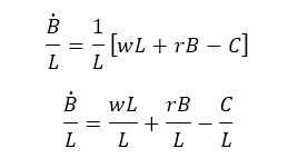
And get to this result.

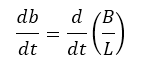
Where b=B/L and c is the consumption in per capita terms. Now we need to find the term with a dot on B/L, and to do this, we use the definition of financial assets in per capita terms given by:

And now we difference respect to time. So, we got.
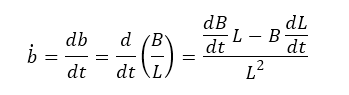
We solve the derivate in general terms as:
And changing the notation with dots (which indicate the variation over time):
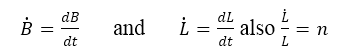
We have
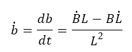
We separate fractions and we got:
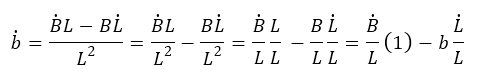
Finally, we have:
Where we going to clear the term to complete our equation derived from the restriction of the families.

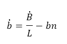
And we replace equation (2) into equation (1). And we have
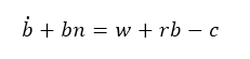
To obtain.

This is the equation to find the evolution of financial assets in per capita terms, where we can see it depends positively on the rate of wages of the economy and the interest rate of returns of the financial assets, meanwhile it depends negatively on the consumption per capita and the growth rate of the population.
The maximization problem of the families is giving then as
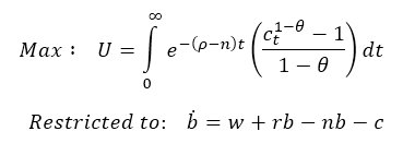
Where we assume that b(0)>0 which indicates that at the beginning of the time, there was at least one existing financial asset.
We need to impose that utility function is limited, so we state:
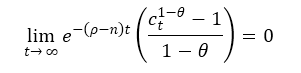
Where in the long run, the limit of utility is going to equal 0.
Now here’s the tricky thing, the use of dynamical techniques of optimization. Without going into the theory behind optimal control. We can use the Hamiltonian approach to find a solution to this maximization problem, the basic structure of the Hamiltonian is the following:
H(.) = Target Function + v (Restriction)
We first need to identify two types of variables before implementing it in our exercise, the control variable, and the state variable. The control variable is the one that focuses on the agent which is a decision-maker, (in this case, the consumption is decided by the individual, and the state variable is the one relegated in the restriction). The state variable is the financial assets or bonus b. Now the term v is the dynamic multiplier of Lagrange, consider it, as the shadow price of the financial assets in per capita terms, and it represents an optimal change in the individual utility given by one extra unit of the assets.
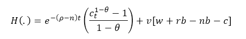
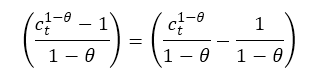
We’re setting what is inside of our integral as our objective, and our restriction remains the same and the Hamiltonian is finally written as:
The first-order conditions are giving by:
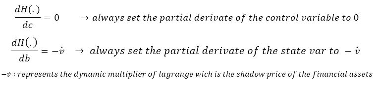
One could ask why we’re setting the partial derivates as this? Well, it’s part of the optimum control theory, but in sum, the control variable is set to be maximized (that’s why it’s equally to 0) but our financial bonus (the state variable) needs to be set negatively to the shadow prices of the evolution of the bonus because we need to find a relationship where for any extra financial asset in time we’ll decrease our utility.
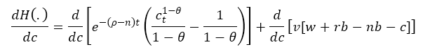
The solution of the first-order condition dH/dc is giving by:
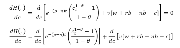
To make easier the derivate we can re-express:
To have now:
Solving the first part we got:
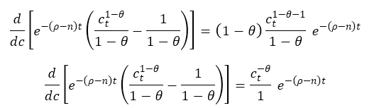
To finally get:
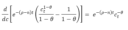
Now solving the term of the first-order condition we obtain:
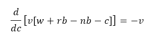
thus the first-order condition is:
Now let’s handle the second equation of first-order condition in dH/db.
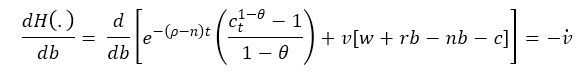
Which is a little bit easier since:
So, it remains:
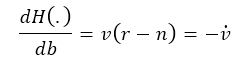
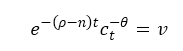
Thus we got.
And that’s it folks, the result of the optimization problem related to the first-order conditions are giving by
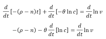
Let’s examine these conditions: the first one is telling us that the shadow price of the financial assets in per capita terms it’s equal to the consumption and the discount factor of the generations within the population grate, some better interpretation can be done by using logarithms. Lets applied them.
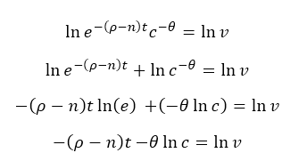
let’s differentiate respect to time and we get:
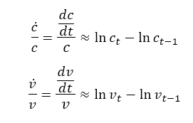
Remember that the difference of logarithms it’s equivalent approximately to a growth rate, so we can write this another notation.
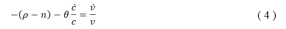
Where
In equation (4) we can identify that the growth rate of the shadow prices of the financial assets is negatively related to the discount rate ρ, and the growth rate of consumption. (in the same way, if you clear the consumption from this equation you can find out that is negatively associated with the growth rate of the shadow prices of the financial assets). Something interesting is that the growth rate of the population is associated positively with the growth in the shadow prices, meaning that if the population is increasing, some kind of pull inflation is going to rise up the shadow prices for the economy.
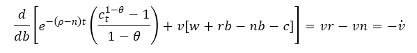
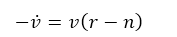
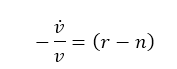
If we multiply (4) by -1, like this
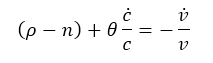
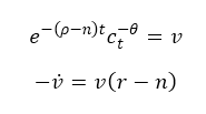
and replace it in the second equation of the first order which is
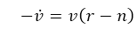
Multiplied by both sides by v, we get
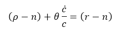
Replacing above equations drive into:
Getting n out of the equation would result in:
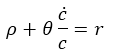
Which is the Euler equation of consumption!
References
Mankiw, N. G., Romer, D., & Weil, N. D. (1992). A CONTRIBUTION TO THE EMPIRICS OF ECONOMIC GROWTH. Quarterly Journal of Economics, 407- 440.
Ramsey, F. P. (1928). A mathematical theory of saving. Economic Journal, vol. 38, no. 152,, 543–559.
Solow, R. (1956). A Contribution to the Theory of Economic Growth. The Quarterly Journal of Economics, Vol. 70, No. 1 (Feb., 1956),, 65-94.
Hello there! This is my 1st comment here so I just wanted to give a quick shout out and tell you I really enjoy reading through your posts. Can you suggest any other blogs/websites/forums that deal with the same subjects? Thanks a ton!
Does your site have a contact page? I’m having trouble locating it
but, I’d like to shoot you an e-mail. I’ve got some ideas for your blog you might be interested in hearing.
Either way, great website and I look forward to seeing
it develop over time.
This excellent website truly has all the information I wanted concerning this subject and didn’t
know who to ask.
A person made some nice factors there. I did a search about the issue as well as discovered nearly just about all individuals goes together with together with your blog.