While modelling specific phenomenon’s in economics, sometimes we might encounter a functional form which may not be linear in the explanatory variables. Assuming, that we still have linearity in the estimators, we have the capability to include in the regression, variables with powers. As an example, consider the following model:

The last equation presents the dependent variable Y as a function of X however, we can see that the polynomial in the model is of second-order degree. A few mentions can be done from here: 1) the model still linear in the parameters β. 2) No multicollinearity can be argued to exists between the regressors in X and the square of X (the model itself in terms of X will be highly correlated) therefore we’re modeling a structure where both of them will move together. 3) The parameters will no longer have a static/basic marginal effect, to find out this marginal effect we need to calculate the derivate of the model, given by:

Which represents that when X increase in one unit, the change in y is the above expression.
Considering the derivate, a turning point is given in the effect of X to Y, and can be found when we equal this derivate to 0 (to find the numerical spot where the slope is equal to 0). And that is done by solving the equation for the value of X:

We clear X and we have:

Let’s see this in practice, first let’s formulate a Data Generating Process -DGP- as follows without any noise or error:

Where X~N(0,1), with Stata let’s generate some random observations and the square variable.
clear all
** Setting observations
set obs 50
gen n=_n
set seed 1234
gen x=rnormal()
gen x_sq=x*x
gen y= 1 + (0.5*x)+ (- 0.2*x_sq)
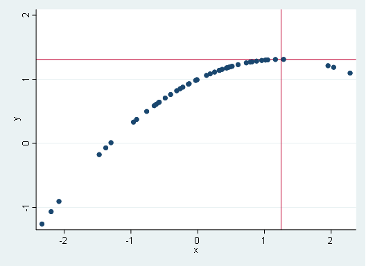
After that, let’s scatter y, over x. and using scatter y x we have the next graph:

If we regress this functional form with the next command:
regress y x x_sq
We have the regression totally adjusted to the DGP. But with missing values on lots of statistics (since there is no residual at all!).
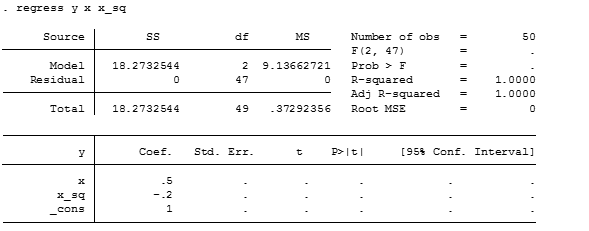
Notice also that the linear adjustment for r-squared is 1, meaning it is matching the data perfectly.
Now confirming that coefficients are 0.5, -0.2 and 1 for the constant. Let’s confirm that the turning point of the model is in:
Solving and changing the parameter’s we have that:

The slope of the curve where it turns to be 0 it should be allocated in X=1.25, with an image in Y=1+0.5(1.25)-0.2(1.25^2)= 1.3125 after that, there’s a decreasing effect in Y given changes in X.
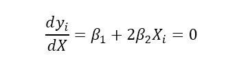
Let’s redo the graph but marking those points.
scatter y x, yline(1.3125) xline(1.25)
We allocated the exact point where the input of x variable is enough to create a decreasing effect on the dependent variable (specifically at x=1.25, y=1.3525) and moving to x>1.25 we have decreasing effects on y, where areas before this point it was positive.
Within this context, let’s introduce to curvefit command.
This package created by Liu wei (2010) and it is good to investigate this kind of nonlinearities, let’s look it in action.
curvefit y x, function(1)
By placing the variables of interest (y as dependent and x as an independent), we need to specify the behavior of the polynomial, as the examples show, function(1) equals a first-order polynomial (a single straight line equation). With the following output.

As you can see, it gives estimates of the coefficients (b0 as the constant with b1 as the slope) and the basic statistic of the number of observations (N) and the adjusted r-squared. The graph displayed is:
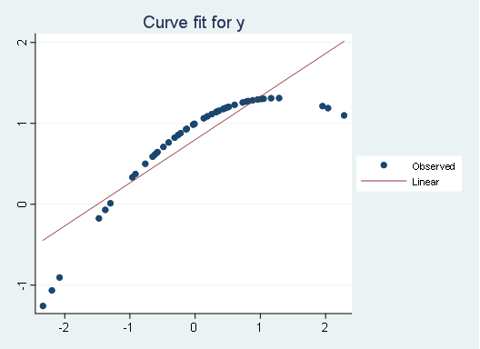
Which is a linear model. A simple regression with first-order power in X. let’s try another function (the quadratic function). We type:
curvefit y x, function(4)
Which gives the following output:

Where b0 is the constant parameter, b1 would equal to the X without any power, and finally, b2 is the parameter associated with X^2. Giving an R^2 adjusted of 1, represents the goodness fit of the model of 100%. With the associated graph:

As you can see, the curve provides estimates pretty decent of the structure of the data given different types of mathematical models.
Here’s the complete list of what kind of functions it can be modeled.
function(string) The following are alternative Models correspond with the values of the sting:

. string = 1 Linear: Y = b0 + (b1 * X)
. string = 2 Logarithmic: Y = b0 + (b1 * ln(X))
. string = 3 Inverse: Y = b0 + (b1 / X)
. string = 4 Quadratic: Y = b0 + (b1 * X) + (b2 * X^2)
. string = 5 Cubic: Y = b0 + (b1 * X) + (b2 * X^2) + (b3 * X^3)
. string = 6 Power: Y = b0 * (X^b1) OR ln(Y) = ln(b0) + (b1 * ln(X))
. string = 7 Compound: Y = b0 * (b1^X) OR ln(Y) = ln(b0) + (ln(b1) * X)
. string = 8 S-curve: Y = e^(b0 + (b1/X)) OR ln(Y) = b0 + (b1/X)
. string = 9 Logistic: Y = b0 / (1 + b1 * e^(-b2 * X))
. string = 0 Growth: Y = e^(b0 + (b1 * X)) OR ln(Y) = b0 + (b1 * X)
. string = a Exponential: Y = b0 * (e^(b1 * X)) OR ln(Y) = ln(b0) + (b1 * X)
. string = b Vapor Pressure: Y = e^(b0 + b1/X + b2 * ln(X))
. string = c Reciprocal Logarithmic: Y = 1 / (b0 + (b1 * ln(X)))
. string = d Modified Power: Y = b0 * b1^(X)
. string = e Shifted Power: Y = b0 * (X - b1)^b2
. string = f Geometric: Y = b0 * X^(b1 * X)
. string = g Modified Geometric: Y = b0 * X^(b1/X)
. string = h nth order Polynomial: Y = b0 + b1X + b2X^2 + b3X^3 + b4X^4 + b5*X^5 …
. string = i Hoerl: Y = b0 * (b1^X) * (X^b2)
. string = j Modified Hoerl: Y = b0 * b1^(1/X) * (X^b2)
. string = k Reciprocal: Y = 1 / (b0 + b1 * X)
. string = l Reciprocal Quadratic: Y = 1 / (b0 + b1 * X + b2 * X^2)
. string = m Bleasdale: Y = (b0 + b1 * X)^(-1 / b2)
. string = n Harris: Y = 1 / (b0 + b1 * X^b2)
. string = o Exponential Association: Y = b0 * (1 - e^(-b1 * X))
. string = p Three-Parameter Exponential Association: Y = b0 * (b1 - e^(-b2 * X))
. string = q Saturation-Growth Rate: Y = b0 * X/(b1 + X)
. string = r Gompertz Relation: Y = b0 * e^(-e^(b1 - b2 * X))
. string = s Richards: Y = b0 / (1 + e^(b1 - b2 * X))^(1/b3)
. string = t MMF: Y = (b0 * b1+b2 * X^b3)/(b1 + X^b3)
. string = u Weibull: Y = b0 - b1*e^(-b2 * X^b3)
. string = v Sinusoidal: Y = b0+b1 * b2 * cos(b2 * X + b3)
. string = w Gaussian: Y = b0 * e^((-(b1 - X)^2)/(2 * b2^2))
. string = x Heat Capacity: Y = b0 + b1 * X + b2/X^2
. string = y Rational: Y = (b0 + b1 * X)/(1 + b2 * X + b3 * X^2)
. string = ALL refers to a total of above models (Attention: it's uppercase!) nograph Curve Estimation without curve fit graph.
This package can be installed using:
ssc install curvefit, replace.
Bibliography.
Liu Wei (2010) “CURVEFIT: Stata module to produces curve estimation regression statistics and related plots between two variables for alternative curve estimation regression models,” Statistical Software Components S457136, Boston College Department of Economics, revised 28 Jul 2013.
I need tto to thank you for this fantastic read!!
I definitely ejoyed every bit of it.I have got you book-marked to
look at new things you post…
Thanks for ones marvelous posting! I quite enjoyed reading it, you might be a great
author. I will always bookmark your blog and will often come
back down the road. I want to encourage continue your great work, have a nice afternoon!
Hello there! Would you mind if I share your blog with my twitter
group? There’s a lott of people that I think would really appreciate your content.Please let me know.
Thanks!
Very good info. Lucky me I discovered your blog by
accident. I have book-marked it for later!
Hello everyone, it’s my first visit at this website, and piece of writing is genuinely fruitful
designedd for me, keep up posting such articles or reviews.
Great delivery. Greatt arguments. Keep up the amazing spirit.
I enjoy reading through your website. Thanks!
Thank you for this very good posts. I was wanting to
know whetherr you were planning oof publishing similar posts to this.
Keep up writing superb content articles!