In this article, we will follow Drukker (2003) procedure to derive the first-order serial correlation test proposed by Jeff Wooldridge (2002) for panel data. It has to be mentioned that this test is considered a robust test, since works with lesser assumptions on the behavior of the heterogeneous individual effects.
We start with the linear model as:

Where y represents the dependent variable, X is the (1xK) vector of exogenous variables, Z is considered a vector of time-invariant covariates. With µ as individual effects for each individual. Special importance is associated with the correlation between X and µ since, if such correlation is zero (or uncorrelated), we better go for the random-effects model, however, if X and µ are correlated, it’s better to stick with fixed-effects.
The estimators of fixed and random effects rely on the absence of serial correlation. From this Wooldridge use the residual from the regression of (1) but in first-differences, which is of the form of:
Notice that such differentiating procedure eliminates the individual effects contained in µ, leading us to think that level-effects are time-invariant, hence if we analyze the variations, we conclude there’s non-existing variation over time of the individual effects.
Once we got the regression in first differences (and assuming that individual-level effects are eliminated) we use the predicted values of the residuals of the first difference regression. Then we double-check the correlation between the residual of the first difference equation and its first lag, if there’s no serial correlation then the correlation should have a value of -0.5 as the next expression states.

Therefore, if the correlation is equal to -.5 the original model in (1) will not have serial correlation. However, if it differs significantly, we have a serial correlation problem of first-order in the original model in (1).
For all of the regressions, we account for the within-panel correlation, therefore all of the procedures require the inclusion of the cluster regression, and also, we omit the constant term in the difference equation. In sum we do:
- Specify our model (whether if it has fixed or random effects, but these should be time-invariant).
- Create the difference model (using first differences on all the variables, therefore the difference model will not have any individual effects). We perform the regression while clustering the individuals and we omit the constant term.
- We predict the residuals of the difference model.
- We regress the predicted residual over the first lag of the predicted residual. We also cluster this regression and omit the constant.
- We test the hypothesis if the lagged residual equal to -0.5.
Let’s do a quick example of these steps using the same example as Drukker.
We start loading the database.
use http://www.stata-press.com/data/r8/nlswork.dta
Then we format the database for stata with the code:
xtset idcode year
Then we generate some quadratic variables.
gen age2 = age^2
gen tenure2 = tenure^2
We regress our model of the form of:
xtreg ln_wage age* ttl_exp tenure* south, fe

It doesn’t matter whether if it is fixed or random effects as long as we assume that individuals’ effects are time invariant (therefore they get eliminated in the first difference model).
Now let’s do the manual estimation of the test. In order to do this, we use a pooled regression of the model without the constant and clustering the regression for the panel variable. This is done of the form:
reg d.ln_wage d.age* d.ttl_exp d.tenure* d.south, noconst cluster(idcode)
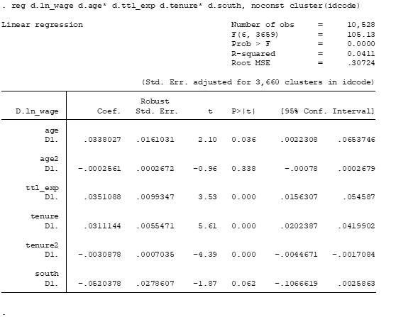
The options noconst eliminates the constant term for the difference model, and cluster option includes a clustering approach in the regression structure, finally idcode is the panel variable which we identify our individuals in the panel.
The next thing to do is predict the residuals of the last pooled difference regression, and we do this with:
predict u, res

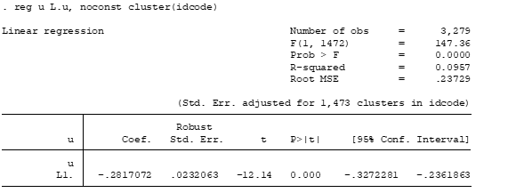
Then we regress the predicted residual u against the first lag of u, while we cluster and also eliminate the constant of the regression as before.
reg u L.u, noconst cluster(idcode)
Finally, we test the hypothesis whether if the coefficient of the first lag of the pooled difference equation is equal or not to -0.5
test L.u==-0.5
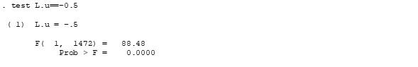
According to the results we strongly reject the null hypothesis of no serial correlation with a 5% level of significance. Therefore, the model has serial correlation problems.
We can also perform the test with the Stata compiled package of Drukker, which can be somewhat faster. We do this by using
xtserial ln_wage age* ttl_exp tenure* south, output

and we’ll have the same results. However, the advantage of the manual procedure of the test is that it can be done for any kind of model or regression.
Bibliography
Drukker, D. (2003) Testing for serial correlation in linear panel-data models, The Stata Journal, 3(2), pp. 168–177. Taken from: https://journals.sagepub.com/doi/pdf/10.1177/1536867X0300300206
Wooldridge, J. M. (2002). Econometric Analysis of Cross Section and Panel Data. Cam-bridge, MA: MIT Press.
Thank you so much for the explanation and for your work. It’s really helpful.
thank you for the feedback !
Hi theгe, I enjoy reading through your post. I wanted to write a little comment to suppοrt you.
thanks for the support!
I absolutely agree with Marisela. I have been looking for a website with straightforward no frills STATA guides written in human language for hours, and finally found one. Please give this man an award and thank you for saving my day Mr. Riveros!
Thank you Mr. Tao! Your comments makes me to put more effort on these monthly articles !
You should take part in a contest for one of the most useful websites online. I’m going to recommend this website!