ARDL model and General to simple methodology

Listening to the word ARDL, the first things that comes into mind is the bound testing approach introduced by Pesaran and Shin (1999).The Pesaran and Shin’s approach is an incredible use of the ARDL, however, the term ARDL is much elder, and the ARDL model has many other uses as well. In fact, the equation used by Pesaran and Shin is a restricted version of ARDL, and the unrestricted version of ARDL was introduced by Sargan (1964) and popularized by David F Hendry and his coauthors in several papers. The most important paper is one which is usually known as DHSY, but we will come to the details DHSY later. Let me introduce what is ARDL and what are the advantages of this model

What is ARDL model?

ARDL model is an a-theoretic model for modeling relationship between two time series. Suppose we want to see the effect of time series variable Xt on another variable Yt. The ARDL model for the purpose will be of the form

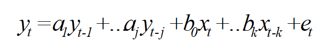
The same model can be written as

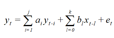
This means, in the layman language the dependent variable is regressed on its own lags, independent variable and the lags of independent variables. The above ARDL model can be termed as ARDL (j, k) model, referring to number of lags j & K in the model.

The model itself is written without any theoretical considerations. However, a large number of theoretical models are embedded inside this model and one can drive appropriate theoretical model by testing and imposing restrictions on the model.

To have more concrete idea, let’s consider the case of relationship between consumption and income. To further simplify, lets consider j=k=1, so that the ARDL(1,1) model for the relationship of consumption and income can be written as

Model 1:          Ct=a+b₁C_t-1+d₀Y_t+d₁Y_t-1+e_t

HereC denotes consumption and Y denotes income, a,b₁,d₀,d₁ denote the regression coefficient and e_t denotes error term. So far, no theory is used to develop this model and the regression coefficients don’t have any theoretical interpretation. However, this model can be used to select appropriate theoretical model for the consumption.

Suppose we have estimated the above mentioned model and found the regression coefficients. We can test any one of the coefficient and/or number of coefficient for various kinds of restriction. Suppose we test the restriction that   

R1: H0: (b₁ d₁)=0

Suppose testing restriction on actual data implies that restriction is valid, this means we can exclude the curresponding variables from the model. Excluding the variables, the model will become

Model 2:          Ct=a+ d₀Y_t+e_t

The model 2 is actually the Keynesian consumption (also called absolute income hypothesis), which says that current consumption is dependent on current income only. The coefficient of income in this equation is the marginal propensity to consume and Keynes predicted that this coefficient would be between 0 and 1, implying that individuals consume a part of their income and save a part of their incomes for future.

Suppose that the data did not suppose the restriction R1, however, the following restriction is valid

R2: H0: d₁=0

This means model 1 would become

Model 3:          Ct=a+b₁C_t-1+d₀Y_t+e_t

This means that current consumption is dependent on current income and past consumption. This is called Habit Persistence model. The past consumption here is the proxy of habit. The model says that what was consumed in the past is having effect on current consumption and is evident from human behavior.

Suppose that the data did not suppose the restriction R1, however, the following restriction is valid

R3: H0: b₁=0

This means model 1 would become

Model 4:          Ct=a+ d₀Y_t+d₁Y_t-1+e_t

This means that current consumption is dependent on current income and past income. This is called Partial Adjustment model. As per implications of Keynesian consumption function, the consumption should only depend on the current income, but the partial adjustment model says that it takes sometimes to adjust to the new income. Therefore, the consumption is partially on the current income and partially on the past income

In a similar way, one can derive many other models out of the model 1 which are representative of different theories. The details of the models that can be drawn from model 1 can be found in Charemza and Deadman (1997)’s ‘New Directions in Econometric Practice…’.  

It can also be shown that the difference form models are also derivable from model 1. Consider the following restriction

R 4:

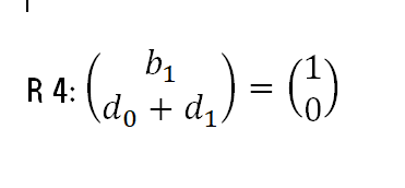
If this restriction is valid, the model 1 will become

Ct=a+C_t-1+d₀Y_t-d₀Y_t-1+e_t

This model can be re-written as

Ct-C_t-1=d₀(Y_t-Y_t-1)+e_t

  This means

Model 5: DCt=d₀DY_t+e_t

This indicates that the difference form models can also be derived from the model 1 with certain restrictions

Further elaboration shows that the error correction models can also be derived from model 1.

Consider model 1 again and subtract C_t-1 both sides, we will get

 Ct- C_t-1=a+b₁C_t-1 -C_t-1+d₀Y_t+d₁Y_t-1+e_t

Adding and subtracting d₀Y_t-1 on the right hand side we get

DCt=a+(b₁-1)C_t-1+d₀Y_t+d₁Y_t-1 +d₀Y_t-1 -d₀Y_t-1 +e_t

DCt=a+(b₁-1)C_t-1+d₀DY_t+d₁Y_t-1 +d₀Y_t-1 +e_t

DCt=a+(b₁-1)C_t-1+d₀DY_t+(d₁+d₀)Y_t-1+e_t

_{This equation contains error correction mechanism if}

R6: (b₁-1)= – (d₁+d₀)

Assume

 (b₁-1)= – (d₁+d₀)=F

The equation will reduce to

DCt=a+F(C_t-1-Y_t-1)+ d₀DY_t +e_t

This is our well known error correction model and can be derived if R6 is valid.

Therefore, existence of an error correction mechanism can also be tested from model 1 and restriction to be considered valid if R6 is valid.  

As we have discussed, number of theoretical models can be driven from model 1 by testing certain restrictions. We can start from model 1 and go with testing different restrictions. We can impose the restriction which is found valid and discard the restrictions which were found invalid in our testing. This provides us a natural way of selection among various theoretical models.

When we say theoretical model, this means there is some economic sense of the model. For example the models 2 to model 6 all make economic sense. So, how to decide between these models? This problem can be solved if we start with an ARDL model and choose to impose restrictions which are permitted by the data

The famous DHSY paper recommends a methodology like this. DHSY recommend that we should start with a large model which encompasses various theoretical models. The model can then be simplified by testing certain restrictions.

In another blog I have argued that if there are different theories for a certain variables, the research must be comparative. This short blog gives the brief outlines about how we can do this. Practically, one need to take larger ARDL structures and number of models that can be derived from the parent model would also be large.