In my the previous blogs, [1] [2] I have explained that following the General Specific Methodology, one can choose between theoretical models to find out a model which is compatible with data. Here is an example which shows step by step procedure of the general to simple methodology.
At the end of this blog, you will find the data on three variables, (i) Household Consumption (ii) GDP and (iii) for the South Korea. The data set is retrieved from WDI
Before starting the modeling, it is very useful to plot the data series. We have three data series, two of them are on same scale and can be plotted together. The third series ‘inflation’ is in percentage form and if plotted with the above mentioned series, it will not be visible. The graph of two series is as follows

You can see, the gap between income and consumption seems to be diverging over time. This is natural phenomenon, suppose a person has income 1000, and consumes 70% of it, the difference between consumption and income would be 300. Suppose the income has gone up to 10,000 and the MPC is same, than the difference between two variables would be widened to 3000. This widening gap is visible in the graph.
However, the widening gap creates problem in OLS. The residuals in the beginning of the data would have smaller variance and at the endpoints, they will have larger variance, i.e. there will be heteroskedasticity. In presence of heteroskedasticity, the OLS doesn’t remain efficient.
The graphs also show a non-linearity, the two series appear to behave like exponential series. A solution to the two problems is to use the log transform. The difference in log transform of two series is roughly equal to the percentage difference, and if the MPC remains same, the gap between two series would be smoothened.
I have taken the log transform and plotted the series again, the graphs is as follows
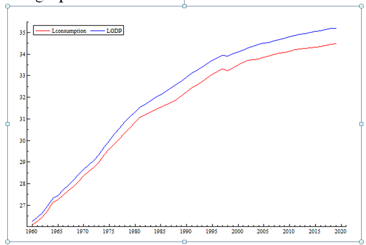
You can see the gap between log transform of two series is smooth compared to the previous graph. One can see the gap is still widening, but much smoother compared to the previous graph. The widening gap in this graph indicates decline in MPC overtime. Anyhow, the two graphs indicate that log transform is better to start building model.
I am starting with ARDL model of the following form

Where Ct indicates consumption Yt and indicates income
The estimated equation is as follows

The equation has very high R-square, but a high R-square in time series is no surprise. This turns out to be high even with unrelated series. However, the thing to note is the sigma which is the standard deviation of residuals, indicating average size of error is 0.0271. Before we proceed further we want to make sure that the estimated model is not having the issue of failure of assumption. We tested the model for normality, autocorrelation and heteroskedasticity, and the results are as follows;

The autocorrelation (AR) test has the null hypothesis of no autocorrelation and the P-value for AR test is above 5%, indicating that the null is no rejected and the hypothesis survived with a narrow margin. Normality test with null of normality and heteroskedasticity test with null of heteroskedasticity also indicate validity of the assumptions.
We want to ensure that the model is also good at prediction, because the ultimate goal of an econometric model is to predict the future. But the problem is, for the real time forecasting, we have to wait for years to see whether the model has the capability to predict. One solution to this problem is to leave some observation out of the model for purpose of prediction and then see how the model works to predict these observations.
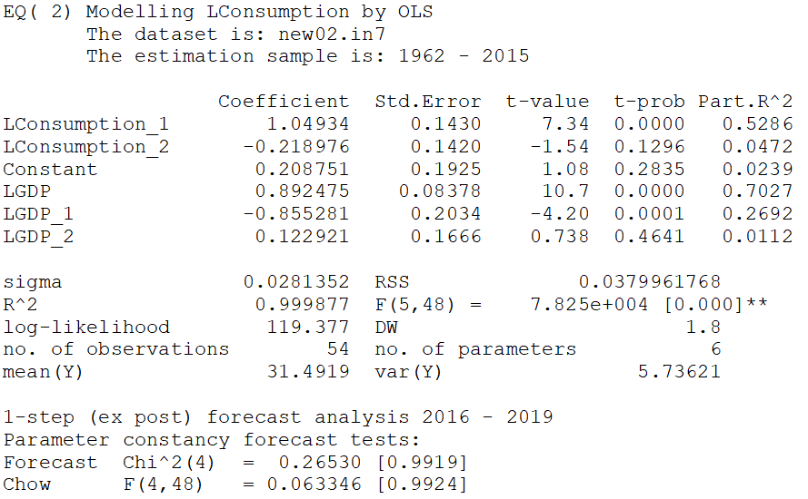
The output indicates that the two tests for predictions have p-value much greater than 5%. The null hypothesis for Forecast Chi-square test is that the error variance for the sample period and forecast period are same and this hypothesis is not rejected. Similarly, the null hypothesis for Chow test is that the parameters remain same for the sample period and forecast period and this hypothesis is also not rejected.

All the diagnostic again show satisfactory results
Now let’s look back at the output of Eq(2). It shows the second lag variables Lconsumption_2 and LGDP_2 are insignificant. This means, keeping the Lconsumption_2 in the model, you can exclude LGDP_2 and vice versa. But to exclude both of these variables, you need to test significance of the two variables simultaneously. Sometime it happens that two variables are individually insignificant but become significant when taken together. Usually this happens due to multi-colinearity. We test joint significance of the two second lag variables, i.e.

The results of the test are
F(2,48) = 2.1631 [0.1260]
The results indicate that the hypothesis is not rejected, therefore, we can assume the coefficients of relevant variables to be zero, therefore the model becomes
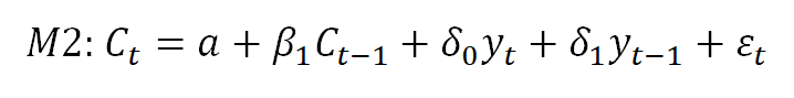
The model M2 was estimated and the results are as follows

The results show the diagnostic tests for the newly estimated model are all OK, and the forecast performance for the new model is not affected by excluding the two variables. If you compare sigma for for Eq (2) and Eq(3), you will the difference only at fourth decimal. This means the size of model is reduced without paying any cost in terms of predictability.
Now the variables in the model are significant except the intercept for which the p-value is 0.178. This means the regression doesn’t support an intercept. We can reduce the model further by excluding intercept. This time we don’t need to test joint restriction because we want to exclude only one variable. After excluding the intercept, the model becomes

The output indicates that all the diagnostic are OK. All the variables are significant, so no variable can be excluded further.
Now we can impose some linear restrictions instead of the exclusion restrictions. For example, if we want to tests whether or not we can take difference of Cons and Income, we need to test following

And if we want to test restriction for the error correction model, we have to test

Apparently the two restriction seems valid because estimated value of is close to 1 and values of sum to 0. We have the choice to test R3 or R4. We are testing restriction R3 first. The results are as follows

This means the error correction model can e estimated for the data under consideration.
For the error correction model, one needs to estimate a static regression (without lags) and to use the residuals of the equation as error correction term. Estimating static regression yield

The estimates of this equation are representative of the long run coefficients of relationship between the two variables. This shows the long run elasticity of consumption with respect to income is 0.93
We have to estimate following kind of error correction regression

The intercept doesn’t enter in the error correction regression. The estimates are as follows

This is the parsimonious model made for the consumption and income. The Eq (5) is representative of long run relationship between two variable and Eq (6) informs about short run dynamics.
The final model has only two parameters, whereas as Eq(1) that we started with contains 6 parameters. The sigma for the Eq(6) and Eq (2) are roughly same which informs that the large model where we started has same predicting power as the last model. The diagnostic tests are all OK which means the final model is statistically adequate in that it the assumption of the model are not opposed by the data.
The final model is an error correction model, which contains information for both short run and long run. The short run information is present in equation (6), whereas the long run information is implicit in the error correction term and it is available in the static Eq (5).
The same methodology can be adapted for the more complex situations and the researcher needs to start from a general model, reducing it successively until the most parsimonious model which is statistically adequate is achieved
Data
Variables Details:
| Consumption: Households and NPISHs Final consumption expenditure (current LCU) |
GDP: GDP Current LCU
Country: Korea, Republic
Time Period: 1960-2019
Source: WDI online (open source data)
| Consumption | GDP | |
| 1960 | 212720000000 | 249860000000 |
| 1961 | 252990000000 | 301690000000 |
| 1962 | 304100000000 | 365860000000 |
| 1963 | 417870000000 | 518540000000 |
| 1964 | 612260000000 | 739680000000 |
| 1965 | 693780000000 | 831390000000 |
| 1966 | 837890000000 | 1066070000000 |
| 1967 | 1039800000000 | 1313620000000 |
| 1968 | 1277060000000 | 1692900000000 |
| 1969 | 1597780000000 | 2212660000000 |
| 1970 | 2062100000000 | 2796600000000 |
| 1971 | 2592400000000 | 3438000000000 |
| 1972 | 3104800000000 | 4267700000000 |
| 1973 | 3798600000000 | 5527300000000 |
| 1974 | 5443600000000 | 7905000000000 |
| 1975 | 7285700000000 | 10543600000000 |
| 1976 | 9315500000000 | 14472800000000 |
| 1977 | 11361500000000 | 18608100000000 |
| 1978 | 15016700000000 | 25154500000000 |
| 1979 | 19439700000000 | 32402300000000 |
| 1980 | 24916700000000 | 39725100000000 |
| 1981 | 31181500000000 | 49669800000000 |
| 1982 | 35278600000000 | 57286600000000 |
| 1983 | 39796800000000 | 68080100000000 |
| 1984 | 44444800000000 | 78591300000000 |
| 1985 | 49305000000000 | 88129700000000 |
| 1986 | 54837200000000 | 102986000000000 |
| 1987 | 61775800000000 | 121698000000000 |
| 1988 | 71362200000000 | 145995000000000 |
| 1989 | 83899400000000 | 165802000000000 |
| 1990 | 100738000000000 | 200556000000000 |
| 1991 | 122045000000000 | 242481000000000 |
| 1992 | 141345000000000 | 277541000000000 |
| 1993 | 161105000000000 | 315181000000000 |
| 1994 | 192771000000000 | 372493000000000 |
| 1995 | 227070000000000 | 436989000000000 |
| 1996 | 261377000000000 | 490851000000000 |
| 1997 | 289425000000000 | 542002000000000 |
| 1998 | 270298000000000 | 537215000000000 |
| 1999 | 311177000000000 | 591453000000000 |
| 2000 | 355141000000000 | 651634000000000 |
| 2001 | 391692000000000 | 707021000000000 |
| 2002 | 440207000000000 | 784741000000000 |
| 2003 | 452737000000000 | 837365000000000 |
| 2004 | 468701000000000 | 908439000000000 |
| 2005 | 500911000000000 | 957448000000000 |
| 2006 | 533278000000000 | 1005600000000000 |
| 2007 | 571810000000000 | 1089660000000000 |
| 2008 | 606356000000000 | 1154220000000000 |
| 2009 | 622809000000000 | 1205350000000000 |
| 2010 | 667061000000000 | 1322610000000000 |
| 2011 | 711119000000000 | 1388940000000000 |
| 2012 | 738312000000000 | 1440110000000000 |
| 2013 | 758005000000000 | 1500820000000000 |
| 2014 | 780463000000000 | 1562930000000000 |
| 2015 | 804812000000000 | 1658020000000000 |
| 2016 | 834805000000000 | 1740780000000000 |
| 2017 | 872791000000000 | 1835700000000000 |
| 2018 | 911576000000000 | 1898190000000000 |
| 2019 | 931670000000000 | 1919040000000000 |