In classic econometrics textbooks and classes, we often associate endogeneity to the correlation or relationship with the error term from a regressor. This is correct and fully agreed upon across authors and professors. But there’s some kind of new endogenous behavior that may not be correlated with the error/residual only, and it may be a situation fully extended away from the classic conception of endogeneity. What I am going to talk to you about in this article is a concept newly discussed in the literature with other names as “Bad Controls” or “Endogenous Co-Regressor” (Cinelli et. al, 2021) and even further mentions in Pearl (2009a, p. 186), Shrier (2009), Pearl (2009c,b), Sj̈olander (2009), Rubin (2009), Ding and Miratrix (2015), and Pearl (2015).
The key to understanding the endogeneity of the co-regressor far away from the classic perspective is derived from the potential covariance which may be different from 0 between the regressors X in a regression model, this produces the topic called “M-Bias” and essentially it is a situation when if one regressor moves, the other regressor do moves too, (slightly different from near-multicollinearity which on the other hand is a linear relationship and not actual changes!).
Let’s start with a linear model as always:

In this setup, we have two regressors which are in notation of matrixes (to simplify the calculous of Least Squares), and we may derive the Least Squares estimator as:
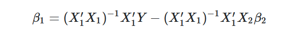
If Cov(X1,X2)= 0 holds, the least-squares estimator for B1 will be unbiased!
Thus, we are interested in the case where the Cov(X1,X2)≠0, a clear implication of the last statement is that when X2 changes also it does change X1. The effect on this will bias the estimates of B1, it creates an “amplification bias effect” because the causal channel is no longer clear in the process to isolate the true effect of X1 on Y.
Notice this is not derived from an existing linear relationship which we may believe from near-multicollinearity, we may define X1=a+bX2+u and this does not necessarily mean that Cov(X1,X2) ≠0, since a linear relationship may exist when two phenomenons are not caused by each other, and X1 must also be potentially endogenous to bias the estimates. Hence, the difference between correlation and causation is important here.
Graphically this means that:
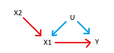
As you can note, X2 is affecting X1 and X1 is also affecting Y, also there may be potential unobserved effects/variables U, which are affecting X1 and Y together. This is the case of the endogenous co-regressor, where X2 is affecting the change on X1, and thus, it will affect the channel effect and amplify the bias if X2 is included in the regression. (This is the case of Model 10 from Cinelli et. al, 2021)
At this point, you may think, “What is this guy talking about? Doesn’t the aggregation of covariates may determine a robust result?” Well, the last is true, but you must be careful to include only sensible covariates and not potential endogenous co-regressors!
In order to demonstrate the effect of this endogenous co-regressor bias amplification, I will follow Cinelli’s Example on R (Cinelli, 2020):
Let’s start creating some observations on R:
n <- 1e5
Now let’s create some random disturbances.
u <- rnorm(n)And now let’s create our regressor x2 with also a random behavior:
x2 <- rnorm(n)Let’s create a Data Generating Process -DGP- where we know that Cov(x1,x2) differs from 0, thus, if X2 changes, it will automatically change X1, making it endogenous:
x <- 2*x2 + u + rnorm(n)And let’s create the DGP for the dependent variable.
y <- x + u + rnorm(n)Notice that y is a linear process that depends on x and u within a randomly distributed disturbance. Hence, the component u (as a disturbance) is affecting both x and y. If we run the regression y over x we will have a biased estimator.
lm(y ~ x)#> Call:
#> lm(formula = y ~ x)
#>
#> Coefficients:
#> (Intercept) x
#> 0.00338 1.16838And one may think, well, we may improve the estimates if we include x2, but look again!
lm(y ~ x + x2) # even more biased#> Call:
#> lm(formula = y ~ x + z)
#>
#> Coefficients:
#> (Intercept) x x2
#> 0.002855 1.495812 -0.985012The coefficient for x has been greatly amplified in the point estimates by the bias-aggregation effect!.
The conclusion of this is that you may double-check again before adding controls on your variables, and be sure to add just sensitive controls, otherwise you will bias the estimates of your regression model!
References:
Cinelli, (2020) Bad Controls and Omitted Variables, Taken from: https://stats.stackexchange.com/questions/196686/bad-controls-and-omitted-variables
Cinelli, C. ; Forney, A. ; Pearl, J. (2021) A Crash Course in Good and Bad Controls, Taken from: https://www.researchgate.net/publication/340082755_A_Crash_Course_in_Good_and_Bad_Controls
Pearl, J. (2009a). Causality. Cambridge University Press
Shrier, I. (2009). Propensity scores. Statistics in Medicine, 28(8):1317–1318.
Pearl, J. (2009c). Myth, confusion, and science in causal analysis. UCLA Cognitive Systems
Laboratory, Technical Report (R-348). URL: https://ucla.in/2EihVyD.
Sjolander, A. (2009). Propensity scores and m-structures. Statistics in medicine,
28(9):1416–1420.
Rubin, D. B. (2009). Should observational studies be designed to allow lack of balance in
covariate distributions across treatment groups? Statistics in Medicine, 28(9):1420–1423.
Ding, P. and Miratrix, L. W. (2015). To adjust or not to adjust? sensitivity analysis of
m-bias and butterfly-bias. Journal of Causal Inference, 3(1):41–57.
Pearl, J. (2015). Comment on ding and miratrix:“to adjust or not to adjust?”. Journal of
Causal Inference, 3(1):59–60. URL: https://ucla.in/2PgOWNd.