
Introduction
In a recent paper from the Journal of Research, Innovation and Technologies published last year, there was a significant discussion (Riveros Gavilanes, 2023) about how control variables might be related to the fulfillment of parallel trends in event study (or dynamic differences-in-differences) of panel data. In this article, we will replicate such paper and present the simple test proposed of parallel pre-trends for differences-in-differences using R. You can also read a copy of this post at r-bloggers.com
The importance of a test far beyond simple averages
The very first thing is to test whether simple averages from the “traditional parallel trend plot” does imply the fulfillment of parallel trends for processes in which both treatment and control groups do follow similar (or equal) trends. For this purpose, we need to run the following code to set up the libraries in R Studio.
| # Packages library (“data.table”) library(“ggplot2”) library(“plm”) library(“lmtest”) #install.packages(“fixest”) library(“fixest”) library(dplyr) #install.packages(“prediction”) library(“prediction”) library(patchwork) library(svglite) |
Then we will set a seed to be able to replicate the exercises.
| set.seed(1) |
The next thing we want to do is to create a simulated panel data (under some significant sample size) which allow us to inspect the dynamics of averages by treatment and control groups.
| Data <- data.table(unit = rep(paste0(“unit”,1:1000), each =10), year =rep(2001:2010, 1000), y = rnorm(10000), treatment = rep(c(1,0), each = 5000)) |
This will create and object from Data Table that will contain 1000 units in a ten year period (2001-2010) sample, where the treatment is simply assigned to the first part of the units. Notice that the dependent variable “y” is normally distributed under default values (mean of 0 and standard deviation of 1)
Then we will simulate a “universal” positive shock (often called universal absorbing treatment) for the year 2005
| # lets start with one specific event that hits in 2005 and # has a positive effect Data[treatment == 1 & year == 2005, y := y + 0.5] |
This shock will be of 0.5 units in the dependent variable only in the year 2005. The rest of the years will remain unaffected, and therefore, they are following the same trend/pattern before the intervention and further than 2006.
The next plot illustrates how the simple average discriminated by treatment and control group can be misleading as the unconditional means do reflect differences in the trends.
| averages <- Data %>% group_by(year, treatment) %>% summarize(avg_y = mean(y)) averages$distance <- averages$year – 2005 averages$group <- ifelse(averages$treatment==1,”Treated”,”Control”) |
This creates an object containing the information inside the data discriminated by the years and the treatment status as a simple average of the dependent variable. Then it creates another variable inside this object to identify whether of they are from the “Treated” or the “Control” group. The next part involves the visualization of the simple or “traditional parallel trend plot”.
| figure1 <- ggplot(averages, aes(x = as.factor(distance), y = avg_y, group = group, color=as.factor(group))) + geom_line() + geom_point() + theme_bw() + geom_vline(xintercept = “0”, linetype = “dashed”, color = “gray”) + labs(x = “Years”, y = “Average Y”, color = “Group”) + ggtitle(“(a) Average Y”) + theme(legend.position = “bottom”, plot.title = element_text(size = 12)) figure1 |
Which shall look like this:
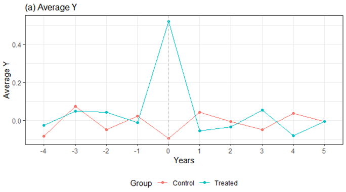
In this case, figure 1 does not display the same trends (especially in periods -3 and -1) where there is a significant difference in the trajectories across groups. This uncontrolled mean calculous reflect how important is to contain for time and unit fixed effects.
The next code instead, shows how the inclusion of fixed effects may alter the dynamics of the model, by using a linear prediction accounting for such effects.
| # Linear trend model Data$post <- 0 Data$post <- ifelse(Data$year>=2005,1,0) Data$post_ind <- Data$post * Data$treatment Data$pre <- 0 Data$pre <- ifelse(Data$year<2005,1,0) # Triple interactions Data$year_t_pre <- Data$treatment*Data$year*Data$pre Data$year_t_post <- Data$treatment*Data$year*Data$post model1 <- plm(y~ post_ind + year_t_pre + year_t_post, data=Data, effect=”twoways”, model=”within”, index=c(“unit”,”year”)) summary(model1) #Prediction of conditional model Dataplm <- pdata.frame(Data, index= c(“unit”,”year”)) Dataplm$predicted <- predict(model1, newdata = Dataplm) #Merge of prediciton Data_plm <- as.data.frame(Dataplm) Data_plm_data <- Data_plm[,c(“unit”,”year”,”predicted”)] Data_plm_data$year <- as.character(Data_plm_data$year) Data_plm_data$year <- as.numeric(Data_plm_data$year) Data_plm_data$unit <- as.character(Data_plm_data$unit) Data <- merge(Data, Data_plm_data, by=c(“unit”,”year”)) Data$predicted <- as.numeric(Data$predicted) Data <- as.data.frame(Data) # Averages of outcomes (Conditional on FE) averages_prediction <- Data %>% group_by(year, treatment) %>% summarize(avg_prediction = mean(predicted)) averages_prediction$distance <- averages_prediction$year – 2005 averages_prediction$group <- ifelse(averages_prediction$treatment==1,”Treated”,”Control”) figure1b <- ggplot(averages_prediction, aes(x = as.factor(distance), y = avg_prediction, group = group, color=as.factor(group))) + geom_line() + geom_point() + theme_bw() + geom_vline(xintercept = “0”, linetype = “dashed”, color = “gray”) + labs(x = “Years”, y = “Predicted Y”, color = “Group”) + ggtitle(“(b) Linear trend model”) + theme(legend.position = “bottom”, plot.title = element_text(size = 12)) figure1b |
The first part of the previous code, set up some dummies for identification: starting by post which is a dummy variable identifying the post-treatment periods in the spirit of differences in differences. The second is “pre” which just identifies the pre intervention. There are some interactions before and after in Data$year_t_pre and Data$year_t_post which allows for a triple time-group specific interaction effects (as part of the linear trends model- which is not very well known usually).
The next part is the estimation of a linear trend model using plm accounting for two ways fixed effects involving the interactions (and of course the time and unit specific effects in the -within- option).
Using this model then we know use a linear prediction to get an estimated of the trends by controlling for these factors before and after for each treated and control group. This done in Dataplm <- pdata.frame(Data, index= c(“unit”,”year”)) and Dataplm$predicted <- predict(model1, newdata = Dataplm) where the prediction is executed.
The other part “ #Merge of prediction” is a messy conversion of the format of the object of pdata into data frame for further manipulation, and finally we go again into the “# Averages of outcomes (Conditional on FE)” to plot the results as figure1b.

Clearly now there is a significant change in the behavior of the trends. To put all together and inspect changes in the trend dyanmics we use:
| combined_plot <- figure1 + figure1b + plot_layout(ncol = 2) combined_plot |
Which looks way too different

This highlights some serious problems. The very first one is that parallel trends may not hold in the simple averages’ calculation whereas accounting for trend or specific fixed effects may do. The second part is that controlling for such effects can be delivering wrongful inferences related to processes in which they hold the same trend. This is evident from this example as the dependent variable follows the same normal distribution for each treated and control unit.
Developing the test based on pre-treatment period significance.
While other alternatives like point specific significance or the Callaway & Sant’Anna estimates provide useful tests, here we are going to stick with the simplest one. And where going to create two dummy variables. But first we need to define the “distance” variable which measures how much away are we each year from the time of the occurrence of the event.
| Data$distance <- Data$year – 2005 |
This will create a general variable which just measures each year in what period are we relative to the event in 2005 (which is the year of the intervention). We move now to the construction of dummies. The key to construct them is to normalize it to a certain point (in this case t=-1) so here goes the first dummy.
| Data$post <- 0 Data$post <- ifelse(Data$distance>= 0,1,0) |
This dummy “post” will be one if whether we are in the year (t=0) of the treatment and onwards, and zero otherwise.
The next dummy is “pre” but be careful, this one shall not take the period (t=-1), instead it should consider the period of pre intervention right before the previous year of the intervention. Therefore, this dummy should be defined from t=-2 and before!
| Data$pre <- 0 Data$pre <- ifelse(Data$distance <= -2 ,1,0) |
Notice how it was constructed? we are implicitly normalizing everything to the period -1, since the pre dummy variable will start to account from t=-2 and before (that is t=-5, t=-4, t=-3 and t=-2) and this dummy will be 1’s and zero otherwise.
Next, we got the interactions with the treatment identificatory:
| # Interactions Data$pre.treatment = Data$pre * Data$treatment Data$post.treatment = Data$post * Data$treatment |
Now the execution of the test must consider using robust standard errors clustered at the unit level. This allows to simply specify a model in the form of:
The estimation of this model by using fixed effects package by Berge (2008) (controls can be added as well) is shown in the following regression output controlling for unit and time fixed effects…
| model1 <- feols(y~ pre.treatment + post.treatment | unit + year, data=Data, cluster=”unit”) summary(model1) |
This red square contains the estimator of the pre*treatment interaction. This is the “parallel trend test-based on pre-treatment period significance” which captures the generic differences between the trends (or trajectories) across the treatment and control groups, relative to the periods of pre intervention stage and referenced to the normalization in period t=-1.

As the parallel pre-trend test is implicit here, the pre*treatment interaction is not statistically significant, therefore suggesting with a p-value of 0.30249, the no rejection of parallel trends between the treatment and control group in the period before the intervention. It must be noted the statistical hypothesis that we are working, in fact H0: β=0 (Null hypothesis of parallel trends in the treatment and control group in the pre-intervention period) against the alternative HA: β ≠0 (Alternative hypothesis of differential trends or trajectories). In this case the coefficient of the interaction pre*treatment is our β of interest.
While the point estimate (β =0.07) can provide some intuition of the deviation of the trends, what is mostly important is the p-value of this coefficient β, (p-value 0.302) where we fail to reject with a 95% level of confidence the null hypothesis of parallel trends in the pre-intervention period.
Final comments
As it was recommended by Riveros Gavilanes (2023), the test ideally should be deployed using event study designs and only in universal absorbing treatments since staggered adoptions may contaminated this test. This complements the testing of parallel pre-trends that potentially may not be true, this in accordance with the statements of Roth (2022) where potentially confounding trends may exist. Therefore, the more tests, the better in this context of parallel trends.
The test proposed here, requires at least 2 pre-treatments periods before the intervention (that is, the year 0 of intervention is mandatory but also year -1 and -2) since all the normalizations occurs in year -1. Therefore, test can only be performed if such 2 pre-treatments periods exist.
Additionally, Riveros Gavilanes (2023) also explores the power of the test under differential sample sizes across treatment and control groups. He suggests that a 1% significance level over the β may be ideal when there is doubt about the parallelism of trends.
Bibliography
Roth, J. (2022). Pretest with caution: Event-study estimates after testing for parallel trends. American Economic Review: Insights, 4(3), 305-322.
Riveros-Gavilanes, J. M. (2023). Testing Parallel Trends in Differences-in-Differences and Event Study Designs: A Research Approach Based on Pre-Treatment Period Significance. Journal of Research, Innovation and Technologies, 2(2 (4)), 226-237. DOI: https://doi.org/10.57017/jorit.v2.2(4).07