Following the last post which gave an example to model the Cobb-Douglas utility function regarding microeconometrics, we need to provide an important aspect related to the behavior of the consumer. That is the budget constraint (referred to as a monetary linear constraint) which limits the number of goods that the consumer can buy and use to get a certain level of utility.
In this article, I want to start with an introduction of the basic concept of budget constrain related to the income in microeconomics, and that’s the linear constraint given a set of quantities and prices of the goods which determine the utility for the consumer, this is closely related to the Cobb-Douglas utility function (and overall utility functions) since it is one of the main aspects of the microeconomic theory.
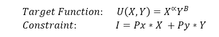
Keeping the utility function as the traditional Cobb-Douglas function:

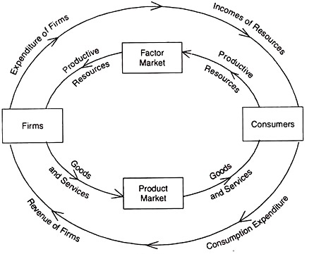
We know that the utility is sensitive to the elasticity αand B. With αand B lesser or equal to one. And since resources are not infinite, we can establish that the amount of goods that the consumer can pay is not infinite. In markets, the only way to get goods and services is with money, and according to the circular flow of the economy, the factor market can revenue two special productive factors: labor and capital, we can say that consumers have a level of income derived from his productive activities.
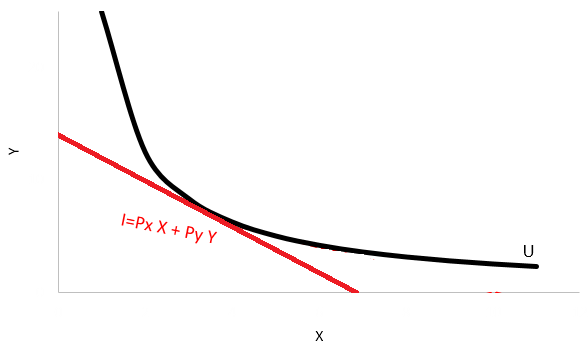
Inside the microeconomic theory in general, utility U is restricted to the income of the consumer within a maximization process with a linear constraint containing the goods and prices which are consumed. The budget constraint for the two good model looks as it follows:

Where I is the income of the individual, Px is the price of the good X and Py is the price of the good Y. One might wonder if the income of the customer is the sum of prices times goods, which doesn’t seem as close to what the circular flows states in a first glance. Income could be defined as the sum of the salary and overall returns of the productive activities (like returns on assets) of the consumer, and there’s no such thing as that in the budget equation.
However, if you look at the equation as a reflection of all the spending on goods (assuming the consumer will spend everything) this will equally match all that he has earned from his productive activities.
The maximization problem of the consumer is established as:
And typical maximization solution is done by using the Lagrange operator where the whole expression of the Lagrange function can be stated as:
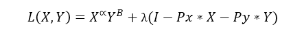
A useful trick to remember how to write this function is to remember that if λ is positive then the income is positive and the prices and goods are negative (we’re moving everything to the left from the constraint equation). And the first-order conditions are given by:
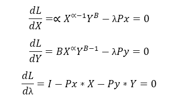
By simply dividing the first two differential equations you’ll get the solution to the consumer’s problem which satisfies the relation as the next ratio:
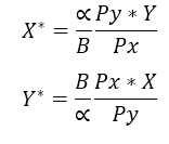
Each good then is primarily sensitive to his own price and the weight (elasticity) in the utility function, seconded by the prices and quantities of the other good Y. If we replace one of the solutions in the last differential equation, say X, we’ll get:
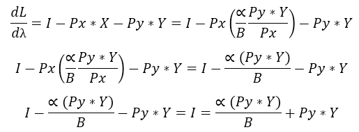
Taking as a general factor the Py*Y will result in:
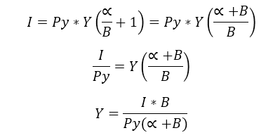
The quantities of the good Y are a ratio of the Income times the elasticity B and this is divided by the price of the same good Y given the sum of the elasticities. Before we stated that α+ B = 1 so we got that B=1- α and the optimum quantities of the goods can be defined now as:
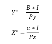
This optimal place its graphically displayed ahead, and it represents the point where the utility is the maximum given a certain level of income and a set of prices for two goods, if you want to expand this analysis please refer to Nicholson (2002).
The budget constrains: An econometric appreciation
Suppose we got a sample of n individuals which only consumes a finite number of goods. The income is given for each individual and also the quantities for each good. How we would be able to estimate the average price that each good has? If we start by assuming that the income is a relation of prices and quantities from the next expression:
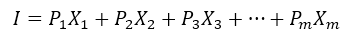
Where X_1 is the good number one associated with the price of the good P_1, the income would be the sum of all quantities multiplicated by their prices or simply, the sum of all expenses. That’s the approach on demand-based income. In this case we got m goods consumed.
Now assume we can replace each price for another variable.
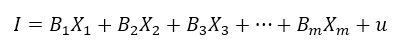
Looks familiar, isn’t it? It’s a regression structure for the equation, so in theory, we are able to estimate each price with ordinary least squares. Assuming as the prices, the estimators associated with each good with B-coefficients. And that all the income is referred to as the other side of the coin for the spending process.
The simulation exercises
Assume we got a process which correlates the following variables (interpret it as the Data Generating Process):
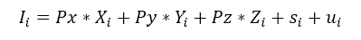
Where I is the total income, Px, Py, Pz are the given prices for the goods X, Y, and Z and we got s which refers to a certain amount of savings, all of this of the individual i. This population according to the DGP not only uses the income for buying the goods X, Y, and Z, but also deposits an amount of savings in s. The prices used in the Monte Carlo approach are Px=10, Py=15, and Pz=20.
If we regress the income and the demanded quantities of each good, we’ll have:
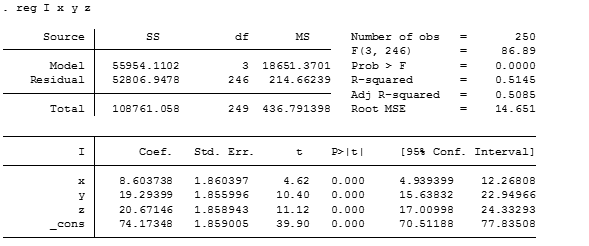
The coefficients don’t match our DGP and that is because our model is suffering from a bias problem related to omitted variables. In this case, we’re not taking into account that the income is not only the sum of expenses in goods but also the income is distributed in savings. Regressing the expression with the s variable we have:
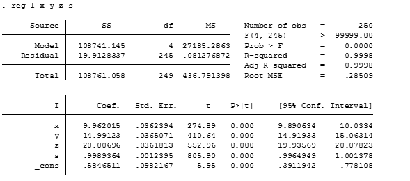
The coefficients for the prices of each good (X, Y, Z) match our DGP almost accurate, R squared has gotten a significant increase from 51.45% to 99.98%. And the overall variance of the model has been reduced. The interesting thing to note here is that the savings of the individuals tend to be associated with an increase in the income with an increase of one monetary unit in the savings.
Remember that this is not an exercise of causality, this is more an exercise of correlation. In this case, we’re just using the information of the goods for the individuals of our sample to estimate the average price for the case of two goods. If we have a misspecification problem, such an approach cannot be performed.
This is one way to estimate the prices that the consumers pay for each good, however, keep in mind that the underlying assumptions are that 1) the prices are given for everyone, they do not vary across individuals, 2) The quantities of X, Y and the amount of savings must be known for each individual and it must be assumed that the spending (including money deposited in savings) should be equivalent to the income. 3) The spending of each individual must be assumed to be distributed among the goods and other variables and those have to be included in the regression, otherwise omitted variable bias can inflict problems in the estimators of the goods we’re analyzing.
References
Kwat, N. (2018). The Circular Flow of Economic Activity. Economics Discussion. Recuperated from: http://www.economicsdiscussion.net/circular-flow/the-circular-flow-of-economic-activity/18159
Marmolejo, I. (2012). Indifference Curve Confusion and Possible Critique. Radical Subjectivist. Recuperated from: https://radicalsubjectivist.wordpress.com/2012/02/10/indifference-curve-confusion-and-possible-critique/
Nicholson, W. (2002). Microeconomic Theory. México D.F.: Thompson Learning.
Highly energetic post, I loved that bit. Will there be a
part 2?
Wonderful blog! I found it while browsing on Yahoo News. Do you have any suggestions on how to get listed in Yahoo News? I’ve been trying for a while but I never seem to get there! Many thanks
I think this is one of the most significant info for me. And i’m glad reading your article. But should remark on some general things, The website style is ideal, the articles is really excellent : D. Good job, cheers
Pretty! This was an incredibly wonderful post.
Thank you for supplying these details.
I just couldn’t depart your web site before suggesting that I extremely enjoyed the standard info a person provide for your visitors? Is gonna be back often to check up on new posts
This post would be much more helpful for beginners if you could provide some background on the Lagrange Operator. And could you please post the Stata code used here as well?
Explaining the Lagrange operator concept will indeed require a new post, however, I might look forward to doing that in the next monthly post. Meanwhile here’s the Stata code used.
clear all
set obs 250
gen s=runiform(50,100)
gen x=round(abs(runiform()))
gen y=round(abs(runiform()))
gen z=round(abs(runiform()))
gen Px=10
gen Py=15
gen Pz=20
gen error=runiform()
gen I=Px*x + Py*y + Pz*z + s + error
reg I x y z
reg I x y z s