While we’re using the time series datasets, often we’re highly likely to find serial correlation and heteroskedasticity in our data. These cases increase the chances to obtain serially correlated errors with non-constant variance.
If we’re purely interested in statistical inferences, we should go for the HAC robust standard errors under the Time Series context. This name as Woolridge appoints refers to:
“In the time series literature, the serial correlation–robust standard errors are sometimes called heteroskedasticity and autocorrelation consistent, or HAC, standard errors.” (Wooldridge, ,p. 432).
We got to appoint that HAC standard errors (also called HAC estimators) are derived from the work of Newey & West (1987) where the objective was to build a robust approach to handle the usual problems of time series associated with serial correlation and heteroskedasticity.
What’s the idea behind these standard errors? Well, we can summarize it as:
- We do not know the form of the serial correlation.
- Works for arbitrary forms of serial correlation and the autocorrelation structure can be derived from the sample size.
- With larger samples, we can be flexible in the amount of serial correlation.
This means, that even when the robust standard error is consistent in the presence of the serial correlation and heteroskedasticity, we still need to figure the lag structure for the autocorrelation. Again, Woolridge helps us to decide this on simple basis:
Annual data = 1 lag, 2 lags. Quarterly data= 4 up to 8 lags. Monthly data = 12 up to 24 lags.
Let’s dig into some formulas to understand the relationship between HAC and OLS.
First, Newey & West standard errors work under the ordinary least squares estimator of the form:

Where X is the matrix of independent variables and Y is the vector of the dependent variable. This leads to establishing that Newey-West estimates in terms of values of the estimators will not differ from the OLS estimates.
Second, Newey & West standard errors modify the role of the estimated variances to include White’s robust approach to heteroskedasticity and also the serial correlation structure.
Consider that estimates of the variance in OLS are given by:

Where Ω is the diagonal matrix containing the distinct variances (for a representation of heteroskedasticity).
Now, White robust estimator is defined by:

Where n is the sample size, and e is the estimated time-period residual with ith row of the matrix of independent variables. Let’s define this as robust estimates with 0 lags (since it is only handling heteroskedasticity).

Now here’s where Newey & West extended the White estimator to include the arbitrary forms of serial correlation with a m-lag structure:

As it is visible, the HAC estimates of the variance now include the heteroskedasticity and a m-lag consistent estimate. K represents the number of independent variables, t the time periods and x is the row of matrix of independent variables observed at time t.
So with this, it is more clearly to work under the frame of :
Annual data: m=1,2 lags. Quarterly data: m=4,8 lags. Monthly data: 12,24 lags.
Let’s see an example:
use https://www.stata-press.com/data/r16/auto
generate t = _n
tsset t
regress price weight displ, vce(robust)

Up to this point, this is the White robust standard errors to heteroskedasticity, now let’s estimate the HAC estimator with the equivalent which is 0 lags.
newey price weight displ, lag(0)
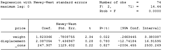
As you can see everything is exact in comparison to the White’s robust standard errors. Now let’s start to use the HAC structure under 2 lags.
newey price weight displ, lag(2)
Notice as well that the values of standard errors of the independent variables have changed with this estimation.

I would recommend always to provide estimates of the HAC SE, in order to obtain more comparative estimates and correct inferences.
As a last mention, Greene (2012) states as a usual practice to select the integer approximate of T^(1/4) where T is the total of time periods of time. For example, for our case considering it is annual data, it would be
display (74)^(1/4)
and Stata will display a value, therefore our lags to select would be 3 and 2 (with no specific criteria to select one over the other).
Bibliography:
Greene, W. H. 2012. Econometric Analysis, 7th edition, section 20.5.2, p. 960
Newey, W. K., and K. D. West. 1987. A simple, positive semi-definite, heteroskedasticity and autocorrelation consistent covariance matrix. Econometrica 55: 703–708.
Wooldridge, J. 2013. Introductory Econometrics: A Modern Approach, Fifth Edition. South-Western CENGAGE Learning.
mind boggling this
You need to take part in a contest for one of the most useful webszites online.
I will recommend this site!
I’m very happy tto discover this page. I need to to thank
you for ones time just for this fantastic read!
I definitely really liked everry little bit of it and I have you bookmarked to check out new things in your blog.
Your mode of describing all in this piece off writing
is in fact pleasant, all be capable of simply be aware of it, Thanks a lot.
Very good post! We wil be linking to this great content on our website.Keep upp the great writing!