Log-linearisation in Short

There exist many different types of models of equations for which there exists no closed form solution. In these cases, we use a method known as log-linearisation. One example of these kinds of models are non-linear models like Dynamic Stochastic General Equilibrium (DSGE) models. DSGE models are non-linear in both parameter and in variables. Because of this, solving and estimating these models is challenging.

Hence, we have to use approximations to the non-linear models. We have to make concessions in this, as some features of the models are lost, but the models become more manageable.

In the simplest terms, we first take the natural logs of the non-linear equations and then we linearise the logged difference equations about the steady state. Finally, we simplify the equations until we have linear equations where the variables are percentage deviations from the steady state. We use the steady state as that is the point where the economy ends up in the absence of future shocks.

Usually in the literature, the main part of estimation consisted of linearised models, but after the global financial crisis, more and more non-linear models are being used. Many discrete time dynamic economic problems require the use of log-linearisation.

There are several ways to do log-linearisation. Some examples of which, have been provided in the bibliography below.

One of the main methods is the application of Taylor Series expansion. Taylor’s theorem tells us that the first-order approximation of any arbitrary function is as below.

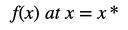
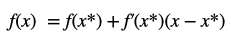
We can use this to log-linearise equations around the steady state. Since we would be log-linearising around the steady state, x* would be the steady state.

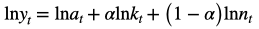
For example, let us consider a Cobb-Douglas production function and then take a log of the function.

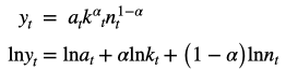
The next step would be to apply Taylor Series Expansion and take the first order approximation.

Since we know that

Those parts of the function will cancel out. We are left with –

For notational ease, we define these terms as percentage deviation of x about x* where x* signifies the steady state.
Thus, we get

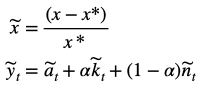
At last, we have log-linearised the Cobb-Douglas production function around the steady state.

Bibliography:
Sims, Eric (2011). Graduate Macro Theory II: Notes on Log-Linearization – 2011. Retrieved from https://www3.nd.edu/~esims1/log_linearization_sp12.pdf

Zietz, Joachim (2006). Log-Linearizing Around the Steady State: A Guide with Examples. SSRN Electronic Journal. 10.2139/ssrn.951753.

McCandless, George (2008). The ABCs of RBCs: An Introduction to Dynamic Macroeconomic Models, Harvard University Press

Uhlig, Harald (1999). A Toolkit for Analyzing Nonlinear Dynamic Stochastic Models Easily, Computational Methods for the Study of Dynamic
Economies, Oxford University Press