Whether if we’re working with Time Series Data or Panel Data, most of the times we want to follow the analysis of the long-run behavior and the short-run dynamics. An interesting but well-known model that enable us for such approach is the Auto-Regressive Distributed Lag model which stands as ARDL. There are a lot of implications regarding the form of the ARDL, maybe some re-parametrizations, maybe some conditional cointegration forms, or fully cointegration equations derived from the ARDL. In this article we’re going to describe how to calculate the long-run coefficient of an ARDL model either for time series or panel data.
Consider the basic Auto-Regressive Distributed Lag model with an exogenous variable, which is of the form:

Where y represents the dependent variable, p represents the autoregressive order of the ARDL, where it is directly associated to the y (the dependent variable). X is an exogenous explanatory variable which has l lags (also a contemporaneous value of x can be included) and the residual term u.
The present form of the ARDL is not actually a long-run form, in fact, it is more a short-run model. Therefore, the actual impact of x through α must be done considering the size and orders associated with the dependent variable y through ß. The above leads to a situation where we want to weigh the cumulative impact of α, and the way to do so is by using a long-run multiplier. Blackburne & Frank (2007) indicate to us that an approximation to this long-run multiplier, would involve a non-linear transformation to get a long-run coefficient, such transformation is given in the general form of:

Where this is the long-run multiplier of the variable X, also please note how this formula works. It’s using the sums of the coefficient α associated to the independent variable (and its lags) divided by 1 minus the sums of the autoregressive ß coefficients. Upper part corresponds to the Long-Run Propensity of X towards y, which is just simply the sums of the coefficients, and it’s interpreted that given one permanent change of one unit in x, the sums would be the long-run propensity as impact on y. The down part represents the weight associated to the response of the autoregressive structure.
This means that if for example, if we got an ARDL (2,2) it refers to a model where we got two lags of the dependent variable and two lags associated to the independent variable (considering of course the contemporaneous value of x). This model is one of the form of

And the weighted long-run multiplier will be given in the form of:

Where α goes from 1 up to 3, it starts from the contemporaneous value of x given by coefficient α1 and then sums the coefficients of the lag orders α2 for lag 1, and α3 for lag 2. Notice that we subtract the sums of the autoregressive parameters ß from the unity to weight the size of the impact of the cumulative sums of x.
Interpretation of the long-run coefficient goes as follow: if x in levels change by one unit, then the average/expected change in y would be given by the long-run coefficient.
Let’s put this together with an example in Stata.
Load up the data base and generate a time identification variable with:
use https://www.stata-press.com/data/r16/auto
generate t = _n
Then tell to Stata that you’re working with time series, so:
tsset t, y
Now let’s estimate an ARDL (2,2) model using the variables of price and weight, where the price is the dependent variable and weight is the independent variable (all assumed to be stationary variables).
reg price L.price L2.price weight L1.weight L2.weight
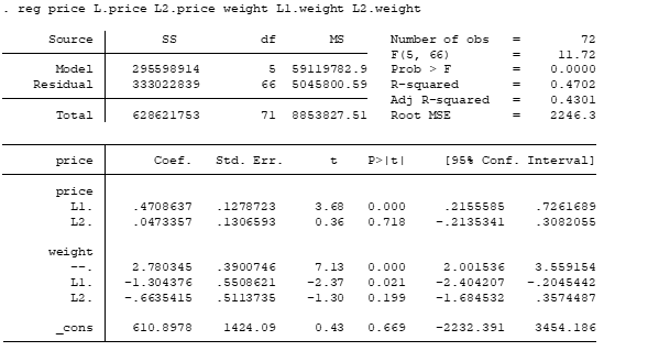
From here you can analyze a lot of things, for example, the long-run propensity will be given by:
** Long-run propensity of x (weight)
display _b[weight] +_b[L1.weight]+_b[L2.weight]

And the long-run multiplier which we discussed, can be calculated by:
** Long-run multiplier of x
display (_b[weight] +_b[L1.weight]+_b[L2.weight]) / (1-(_b[L1.price] + _b[L2.price]))

And from here, you can even go to estimate the long-run coefficient with statistical significance and the actual value of the long-run coefficient by using nlcom: this can be done by using:
nlcom (_b[weight] +_b[L1.weight]+_b[L2.weight]) / (1-(_b[L1.price] + _b[L2.price]))

Notice that when the weight increases in unit over the long-run the expected change would be of 1.68 units on the price, statistically significant with a 10% level of significance.
You can extend such analysis to the famous long-run & short-run dynamics of the Cointegration tests of Engle & Granger, where you just will have to compute the short-run coefficients in order to obtain the long-run coefficients, this will be done in a future next post.
An excellent video to help you to get this idea can be found in Nyboe Tabor (2016).
Bibliography:
Blackburne, E. F. & Frank, M.W. (2007) Estimation of nonstationary heterogeneous panels The Stata Journal (2007), 7, Number 2, pp. 197-208.
Nyboe Tabor, M. (2016) The ADL Model for Stationary Time Series: Long-run Multipliers and the Long-run Solution, Recuperated from: https://www.youtube.com/watch?v=GLpCVrZbW-g
Can you please provide a PhD topic on ARDL for me
I a newly admitted student in to the university n Nigeria.
Excellent piece by @John M. Riveros. I was planning to write a similar thing myself, but it better.
Thank you kindly for your comments Dr. Rehman